Open SourceSep 3, 2025

Turn Jupyter Notebooks into Production Dashboards in Python

Convert Jupyter notebooks into production-ready dashboards with Reflex. Keep your pandas logic, add UI components, and deploy.

The Data Scientist's Dilemma

Data scientists excel at analysis but struggle with productionization. You build sophisticated models in Jupyter notebooks, then face the dreaded request: "Can we make this a live dashboard?"

The usual options aren't great. Hand it off to engineers and wait months. Use limited dashboard tools that can't handle your analysis complexity. Or learn React, APIs, and deployment just to make your Python work interactive.

This guide shows a different path: transforming your Jupyter analysis directly into a production dashboard without leaving Python.

Our Starting Point: The Jupyter Notebook

Let's work with a realistic scenario: analyzing customer churn using the IBM Telco dataset. Here's what a typical analysis notebook looks like:

import pandas as pd
import numpy as np
import matplotlib.pyplot as plt
import seaborn as sns
from sklearn.ensemble import RandomForestClassifier

# Load the IBM Telco customer churn dataset
url = "https://raw.githubusercontent.com/IBM/telco-customer-churn-on-icp4d/master/data/Telco-Customer-Churn.csv"
df = pd.read_csv(url)

print(f"Dataset shape: {df.shape}")

# Prepare columns and add some realistic features
df['last_login'] = pd.to_datetime("2022-01-01") + pd.to_timedelta(np.random.randint(0, 400, len(df)), unit='D')
df['usage_last_30d'] = np.random.randint(10, 500, len(df))
df['usage_prev_30d'] = np.random.randint(10, 500, len(df))
df['support_tickets'] = np.random.poisson(2, len(df))
df['plan_value'] = df['MonthlyCharges']
df['plan_type'] = df['Contract']
df['churned'] = df['Churn'].map({'Yes': 1, 'No': 0})

print(f"Churn rate: {df['churned'].mean():.2%}")

# Feature engineering
df['days_since_last_login'] = (pd.Timestamp.now() - df['last_login']).dt.days
df['usage_decline'] = df['usage_last_30d'] / (df['usage_prev_30d'] + 1e-5)

# Key insights
churn_by_plan = df.groupby('plan_type')['churned'].agg(['count', 'mean'])
print("\nChurn by Plan Type:")
print(churn_by_plan)

# Visualizations
fig, axes = plt.subplots(2, 2, figsize=(12, 8))

churn_by_plan['mean'].plot(kind='bar', ax=axes[0,0], title='Churn Rate by Plan')
df.boxplot('usage_decline', by='churned', ax=axes[0,1])
axes[0,1].set_title('Usage Decline: Churned vs Active')
df.hist(column='days_since_last_login', by='churned', bins=20, ax=axes[1,0])
axes[1,0].set_title('Days Since Last Login Distribution')
sns.histplot(data=df, x='plan_value', hue='churned', kde=True, ax=axes[1,1])
axes[1,1].set_title('Plan Value Distribution')

plt.tight_layout()
plt.show()

# Predictive model
features = ['days_since_last_login', 'usage_decline', 'support_tickets', 'plan_value']
X = df[features]
y = df['churned']

rf = RandomForestClassifier(random_state=42)
rf.fit(X, y)

print(f"\nModel accuracy: {rf.score(X, y):.3f}")
print("Feature importance:")
for feature, importance in zip(features, rf.feature_importances_):
    print(f"  {feature}: {importance:.3f}")

Expand

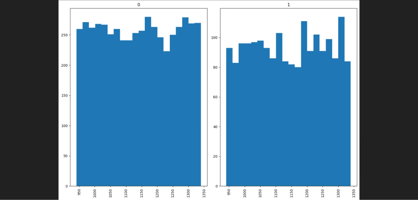
Interactive plots in a Reflex Jupyter dashboard

Plots generated from Google Colab using Jupyter Notebook

This notebook does what data scientists do every day: loads data, engineers features, explores patterns, and builds predictive models. The analysis works, the insights are valuable, but it's stuck in a static format.

When stakeholders ask "Can we see this updating with fresh data?" you're back to the productionization problem.

The Productionization Problem

Your notebook analysis is solid, but it has limitations. The plots are static images. The insights are buried in print statements. To see updated results, someone needs to rerun the entire notebook manually.

Traditional solutions force you to choose between complexity and capability:

Flask + React: Build a backend API, create React components, manage state, handle authentication. Weeks of work to recreate what you already built.

Streamlit: Quick to deploy, but limited interactivity. Complex analyses don't translate well to Streamlit's widget-based approach.

Hand-off to engineering: Wait months while engineers rebuild your analysis, often losing nuance in translation.

None of these options preserve your existing work or let you iterate quickly. What if you could keep your Python analysis logic and just make it interactive?

Transforming to Reflex

Here's how to transform our notebook into an interactive dashboard. Your data processing logic stays the same—we just add Reflex components around it.

Project Structure

First, let's set up a proper Reflex project structure:

churn-dashboard/
├── app/
│   ├── __init__.py
│   ├── app.py
│   ├── state.py
│   └── components/
│       ├── __init__.py
│       ├── kpi_card.py
│       └── bar_chart.py
├── assets/
├── requirements.txt
└── rxconfig.py

Step 1: State Management (app/state.py)

Move your notebook's data processing logic into a Reflex state class:

import reflex as rx
import pandas as pd
import logging
import asyncio


class DashboardState(rx.State):
    """The app state."""

    is_loading: bool = True
    total_customers: int = 0
    total_churn: int = 0
    churn_rate: float = 0.0
    avg_monthly_charges: float = 0.0
    churn_by_contract: list[dict[str, str | int]] = []
    churn_by_tenure: list[dict[str, str | int]] = []
    chart_view: str = "Contract"

    @rx.event(background=True)
    async def load_data(self):
        """Load and process the data from the URL."""
        async with self:
            self.is_loading = True
        try:
            await asyncio.sleep(0.5)
            url = "https://raw.githubusercontent.com/IBM/telco-customer-churn-on-icp4d/master/data/Telco-Customer-Churn.csv"
            df = pd.read_csv(url)
            df["TotalCharges"] = pd.to_numeric(df["TotalCharges"], errors="coerce")
            df.dropna(inplace=True)
            total_customers = len(df)
            total_churn = len(df[df["Churn"] == "Yes"])
            churn_rate = (
                total_churn / total_customers * 100 if total_customers > 0 else 0
            )
            avg_monthly_charges = df["MonthlyCharges"].mean()
            churn_data_contract = (
                df.groupby("Contract")["Churn"].value_counts().unstack(fill_value=0)
            )
            churn_data_contract.reset_index(inplace=True)
            churn_data_contract.rename(
                columns={"No": "retained", "Yes": "churned"}, inplace=True
            )
            chart_data_contract = churn_data_contract.to_dict(orient="records")
            bins = [0, 12, 24, 36, 48, 60, df["tenure"].max()]
            labels = ["0-12m", "13-24m", "25-36m", "37-48m", "49-60m", "61m+"]
            df["tenure_group"] = pd.cut(
                df["tenure"], bins=bins, labels=labels, right=True, include_lowest=True
            )
            churn_data_tenure = (
                df.groupby("tenure_group", observed=False)["Churn"]
                .value_counts()
                .unstack(fill_value=0)
            )
            churn_data_tenure.reset_index(inplace=True)
            churn_data_tenure.rename(
                columns={"No": "retained", "Yes": "churned"}, inplace=True
            )
            chart_data_tenure = churn_data_tenure.to_dict(orient="records")
            async with self:
                self.total_customers = total_customers
                self.total_churn = total_churn
                self.churn_rate = round(churn_rate, 2)
                self.avg_monthly_charges = round(avg_monthly_charges, 2)
                self.churn_by_contract = chart_data_contract
                self.churn_by_tenure = chart_data_tenure
                self.is_loading = False
        except Exception as e:
            logging.exception(f"Failed to load data: {e}")
            async with self:
                self.is_loading = False

    @rx.event
    def set_chart_view(self, view: str):
        self.chart_view = view

    @rx.var
    def chart_data(self) -> list[dict[str, str | int]]:
        if self.chart_view == "Contract":
            return self.churn_by_contract
        return self.churn_by_tenure

    @rx.var
    def chart_title(self) -> str:
        if self.chart_view == "Contract":
            return "Customer Retention by Contract Type"
        return "Customer Retention by Tenure"

    @rx.var
    def chart_x_axis_key(self) -> str:
        if self.chart_view == "Contract":
            return "Contract"
        return "tenure_group"

Expand

Step 2: Chart Component (app/components/bar_chart.py)

Convert your matplotlib bar chart to an interactive Reflex chart:

import reflex as rx
from app.state import DashboardState

def churn_bar_chart() -> rx.Component:
    """A bar chart showing churn by contract type."""
    return rx.el.div(
        rx.el.h3("Customer Retention by Contract Type"),
        rx.recharts.bar_chart(
            rx.recharts.cartesian_grid(vertical=False),
            rx.recharts.x_axis(data_key="Contract"),
            rx.recharts.y_axis(),
            rx.recharts.legend(),
            rx.recharts.bar(
                data_key="retained",
                name="Retained",
                fill="#3b82f6",
                stack_id="a"
            ),
            rx.recharts.bar(
                data_key="churned",
                name="Churned",
                fill="#ef4444",
                stack_id="a"
            ),
            data=DashboardState.churn_by_contract,
            height=300,
        )
    )

Expand

Step 3: KPI Cards (app/components/kpi_card.py)

Create reusable metric cards to replace your print statements:

import reflex as rx

def kpi_card(title: str, value: str | int, icon: str, color: str) -> rx.Component:
    """A reusable KPI card component."""
    return rx.el.div(
        rx.el.div(
            rx.icon(icon, class_name="w-6 h-6"),
            class_name=f"p-3 rounded-full {color}"
        ),
        rx.el.div(
            rx.el.p(title, class_name="text-xs font-medium text-gray-500"),
            rx.el.p(value, class_name="text-xl font-semibold text-gray-800"),
        ),
        class_name="flex items-center gap-4 p-4 bg-white border border-gray-200 rounded-xl shadow-sm",
    )

Step 4: Main Dashboard (app/app.py)

Bring everything together into a dashboard:

import reflex as rx
from app.state import DashboardState
from app.components.kpi_card import kpi_card
from app.components.bar_chart import churn_bar_chart

def index() -> rx.Component:
    """The main dashboard page."""
    return rx.el.main(
        rx.el.div(
            rx.el.h1("Telco Churn Dashboard"),

            # KPI Cards - replacing our print statements
            rx.el.div(
                kpi_card("Total Customers", DashboardState.total_customers, "users", "bg-blue-100 text-blue-600"),
                kpi_card("Total Churn", DashboardState.total_churn, "user-minus", "bg-red-100 text-red-600"),
                kpi_card("Churn Rate", f"{DashboardState.churn_rate}%", "trending-down", "bg-yellow-100 text-yellow-600"),
                kpi_card("Avg Monthly Bill", f"${DashboardState.avg_monthly_charges}", "dollar-sign", "bg-green-100 text-green-600"),
                class_name="grid grid-cols-1 sm:grid-cols-2 lg:grid-cols-4 gap-4",
            ),
            # Chart - replacing our matplotlib plot
            churn_bar_chart(),
        ),
        on_mount=DashboardState.load_data,
    )

app = rx.App()
app.add_page(index)

Expand

Your notebook's pandas analysis logic stays intact, it just moves into the load_data method. The static matplotlib plots become interactive charts, and your print statements become clean KPI cards. The same insights, now accessible to anyone with a web browser.

If you want to try this dashboard live, you can do so here on Reflex Build -> Churn Dashboard

You can edit, re-work, and improve it as you see fit!

Deploying with Reflex

The final step is sharing your work. A dashboard is only valuable if others can access it, and deployment is where most data science projects stall.

With Reflex, deployment is built-in. You don’t need to worry about servers, Docker, or frontend builds. Your Python app can be published live with a single command:

reflex deploy

For detailed information on how deployment works, visit the Cloud Deploy Docs to find out how to begin.

Wrapping Up

We started with a Jupyter notebook full of exploratory analysis—static plots and printouts that lived on your laptop. Then, we showed how to transform that work into a production-grade dashboard with Reflex, keeping your Python workflow intact. Finally, we saw how easy it is to deploy and share your dashboard.

With this workflow, data scientists can go from notebook → live dashboard → deployed app in hours instead of weeks.

Next steps: